Machine Learning Techniques for Predictive Maintenance

Decision trees

This is probably one of the most powerful tools for prediction and classification. It looks like a tree structure, where each internal node denotes a test on an attribute, the outcome of the test is being represented by each branch, and each leaf node (terminal node) holds a class label.

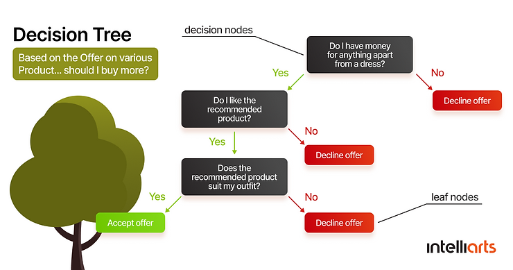
To build a tree, we need to divide a source set into subsets based on the attribute value test. This is a repeatable process for each derived subset in a recursive manner and is called recursive partitioning. When the subset at a node has the same value of the target available, or in a case when splitting no longer adds value to the forecasts, the recursion is considered complete. You don’t need any domain knowledge or parameter setting to build a decision tree classifier, hence it’s suitable for exploratory knowledge discovery.

How to use trees in PdM?

There are plenty of interesting use cases, let’s focus on two of them.

Case 1: Fault diagnosis and detection in grid-connected photovoltaic systems (GCPVS)

GCPVS are electricity-generating solar PV power systems that are connected to the utility grid. A grid-connected PV system consists of solar panels, one or multiple inverters, a power conditioning unit, and grid connection equipment. The grid-connected PV system supplies the excess power, beyond consumption by the connected load, to the utility grid, saving on the electricity bills for the customer. However, without proper maintenance, the whole point of these devices will be missed, because they won’t operate correctly.

According to the case described by Rabah Benkercha and Samir Moulahoum, a decision tree algorithm was used to detect faults in GCPVS. To complete this goal, a non-parametric model was implemented to forecast the state of GCVPS, and the dataset was collected from GCPVS by the acquisition system in different weather conditions. The data used for model training consisted of three numerical attributes and two targets.

The attributes included:

• Temperature ambient

• Irradiation

• Power ratio (calculated from measured and estimated power)

The targets included:

• Healthy or faulty state for detection

• Four classes of labels for diagnosis: free fault, string fault, short circuit fault, or line-line fault

Additionally, the Sandia model was chosen to estimate the power produced by GCPVS during the healthy state of operation (in 2015 Sandia has developed a software toolkit that uses stochastic programming to perform power system production cost model simulations, which was named PRESCIENT). All collected data was split into two parts, 66% of which were used for learning and the remaining part was used for testing.

The new data was recorded for five days in total in order to evaluate both models robustness and efficiency. The results were very impressive, as the decision trees model used for the diagnosis task was able to reach 99.80% of accuracy. The Sandia model evaluation showed high prediction accuracy, with the correct classification number being close to 100%.

Case 2: Determining RUL of lithium-ion batteries

Another interesting case of leveraging decision trees is finding out the remaining useful life (RUL) of lithium-ion batteries. These batteries can only be used in specific conditions and require a battery management system (BMS) to monitor the battery state to ensure the safety of the operation.

Multiple machine learning techniques for predictive maintenance were applied to deal with RUL challenges, but they faced the following limitations:

• The extracted features didn’t reflect the information hidden in the historical degradation status

• Nonlinearity caused imprecise OR low accuracy of battery degradation prediction

One of the options to solve this was to combine the time window (TW) and gradient boosting decision trees (GBDT). In this method, the energy and fluctuation index of voltage signals were being verified and chosen as features. After that, a time window-based method was used to extract features from the historical discharge process. The next step was to adopt gradient boosting decision trees for modeling the relation of features and remaining useful life. This method has proven results to solve this problem.

Support vector machines (SVM)

This is a model that fits great for classification and regression problems. It can solve linear and non-linear problems and works well for a variety of other real-world problems. The algorithm creates a line or a hyperplane which separates the data into two classes:

The key idea of this algorithm is to find a hyperplane in N-dimensional space (in which N represents the number of features) that distinctly classifies the data points. Among two classes of data points, a lot of possible hyperplanes can be chosen. The goal is to find a hyperplane with a maximum margin, or the maximum distance between data points of both classes. The future data points can be classified with more confidence when the margin distance will be maximized. To provide you context, let’s review some applications of SVM in predictive maintenance.

Case 1: Fault detection and diagnosis of chillers

The first case is a classification problem that implements fault detection and diagnosis (FDD) of chillers. The chillers are used in buildings to provide cooling and are often the most energy-consuming piece of equipment.

In one of the cases, the least squares support vector machine (LS-SVM) model was additionally optimized by cross-validation to leverage FDD on a 90-ton centrifugal chiller. To achieve the goal, three system-level and four component-level faults were analyzed. A detailed discussion was conducted to validate and employ eight fault-indicative features extracted from the original 64 parameters. Compared with the other two machine learning methods used in this project, the LS-SVM model showed better results in the following parameters, especially those on the system level:

• overall diagnostic efficiency

• detection rate

• false alarm rate

The prediction precision was quite impressive, with refrigerant leak/undercharge (99.59%), refrigerant overcharge (99.26%), and excessive oil (99.38%).

Case 2: Another RUL estimation

Going back to remaining useful life estimation, there was a case when it was needed to estimate the RUL directly from sensor values, without estimating degradation states or failure threshold. Sometimes it is important to be able to estimate RUL at any stage of the degradation process.

To achieve this goal, a direct relation between sensor values was modeled with the help of support vector regression (SVR). This is the most popular approach for fault prognosis. The experimental results showed that the SVR approach is a viable alternative to the existing methods. Not only RUL can be estimated at any point of the degradation process, but also an offline wrapper variable selection can be applied before training the prediction model (which reduces computational time and increases accuracy).

K-Nearest neighbors algorithm (KNN)

This is a supervised machine learning algorithm in predictive maintenance that can deal with both classification and regression problems. KNN algorithm works in the way that similar data points are close to each other. The algorithm finds the distances between a query and all the examples in the data and selects the specified number of examples (K) closest to the query. After that, the algorithm votes for the most frequent label, if we talk about classification. For the regression problem, the averages of labels are being calculated. When the new data appears, it is classified in one of the categories. Let’s say we have Class A, Class B, and the new unknown data point “?”. This data point is classified by a majority vote of the neighbors and assigned to the class most common amongst its K nearest neighbors, which is measured by a distance function.

In other words, KNN is all about similarity (also known as closeness, distance, or proximity) and calculating the distance between points on a graph. Moving to practical implementation in predictive maintenance, there are a few cases worth our attention.

Case 1: The diagnosis of electric traction motors

First, the automotive industry has a wide application for electric traction motors. The operational conditions of these motors could be characterized by variable load, rotational speed, and other external conditions which complicate the process of diagnosing bearing defects. Because of this, there is a challenge for detecting the onset of degradation, isolating the degrading bearing, and making a classification of defect types.

This is a classification problem that was solved by leveraging a diagnostic system built based on a hierarchical structure of K-nearest neighbors classifiers. Previously measured vibrational signals were used as input. The bearing diagnostic system was done by an approach that was based on multi-objective (MO) optimization that integrates a binary differential evolution (BDE) algorithm with the KNN classifiers. While this approach was applied to the experimental dataset, the results showed the capabilities of this method to solve the issue.

Case 2: Improving the reliability of insulated gate bipolar transistor

As an example of a regression problem, we can talk about an insulated gate bipolar transistor (IGBT), which is a great performance switching device commonly used in power electronic systems. However, there is a challenge in ensuring reliability and safety for IGBT, which KNN can solve.

There is an innovation in this field, as a new prediction model with a complete structure based on an optimally pruned extreme learning machine (OPELM) and Volterra series is recommended to predict the remaining useful life of insulated gate bipolar transistor and forecast its degradation. We can refer to this model as the Volterra k-nearest neighbor OPELM prediction (VKOPP) model. The model needs the minimum entropy rate method and Volterra series to rebuild phase space for IGBT’s aging samples. The new version of the algorithm can effectively reduce the negative impact of noises and outliers and is used to establish the VKOPP network. To successfully forecast remaining useful life for the IGBT the combination of the K-Nearest Neighbors method and least squares estimation (LSE) is leveraged to calculate the output weight of OPELM.

Compared to the classic prediction approaches, the prognostic results show that this one can predict the RUL of IGBT modules with small error, lower time spending, and significantly higher precision.

Obviously, there is no single perfect approach to solving each particular challenge. Each algorithm that we mentioned in the article, has its best area for implementation. Let’s take a look at the pros and cons of each specific algorithm.

Decision trees

Advantages:

• Significantly less effort in data preparation during pre-processing phase compared to other algorithms

• Do not require data normalization

• Do not require data scaling

• Missing values are not a major or disrupting problem for building a decision tree

• Very intuitive and easy to understand and explain to your developers and business partners

Disadvantages:

• Possible instability due to the smallest change in data that cause major changes in the decision tree structure

• Sometimes require much more complex calculations compared to other existing algorithms

• Decision trees are relatively more expensive and time-consuming in training

• Are not suitable for solving regression problems or predicting continuous values

Support vector machines (SVM)

Advantages:

• Work well even with unstructured and semi-structured data

• Have less risk of overfitting

• Work relatively well in scenarios with a clear margin of separation between classes

• Much more effective in high-dimensional spaces

• Very effective in scenarios where the amount of dimensions is higher than the number of samples

• Relatively memory efficient compared to other algorithms

Disadvantages:

• No probabilistic explanation for the classification

• No standard for choosing the kernel function

• Not suitable for massive sets of data

• Do not perform well when the data has a big amount of noise and target classes are overlapping

• Will underperform in scenarios when the number of features of each data point will exceed the number of training data samples

K-Nearest neighbors algorithm (KNN)

Advantages:

• Zero time for training. KNN is often called lazy learner or instance-based learning. Because the algorithm doesn’t learn during the training period and does not derive any discriminative function from data, we can consider that it doesn’t have a training period. It has a storage of training datasets and learns only when making real-time predictions. This feature makes this algorithm faster than the other alternatives that require training.

• Seamless adding of the new data. Because the KNN algorithm doesn’t need training before actual prediction generation, you can add new data easily, and it will not impact the overall accuracy in any way.

• Ease of implementation. To make it work, you only need two parameters, the value of K and the distance function.

Disadvantages:

• It is not the best option for a large dataset, because the final cost of determining the distance between the new point and each of the existing points will be massive and will decrease the performance level of the algorithm dramatically.

• Not the best option for multiple dimensions. Once again, with a big number of dimensions KNN algorithm won’t work well, because of the need to calculate the distance in each dimension.

• Requires feature scaling. The feature scaling, standardization, and normalization are mandatory before applying the algorithm to any dataset. Without this move, there is a risk for KNN algorithm to make wrong predictions in the end.

• “K” in the algorithm must be determined in advance

• The algorithm is very sensitive to the unbalanced datasets

• Too sensitive to missing values, outliers, and noisy data. With the KNN algorithm, we can’t allow noise in the dataset. All missing values must be added and outliers removed manually to make the algorithm work properly.

In the article, we highlighted the three most popular machine learning algorithms to solve a predictive maintenance challenge across various industries. As you see, there is no ultimate solution that will fit any situation like a glove. A proper algorithm must be chosen carefully and rigorously, based on your specific problem, available dataset, time and budget, and your business goals. While machine learning technology offers very powerful techniques for predictive maintenance challenges, they are far from perfect and have their own limitations and disadvantages. In most cases, you need meaningful data that is properly collected and processed in the right way to build the ML solution for a hydraulic system.

The best option is to contact a team of experienced machine learning experts and get their help with evaluating your business situation, conducting a discovery phase to see what solution you have at the moment, building a data collection pipeline, and, if all required conditions are met, developing a custom predictive maintenance solution that can save your organization an enormous amount of money and resources.

Follow our articles and get all the insights, as we continue to share our experience on advanced machine learning techniques, including automated data extraction from PDF, which can transform unstructured data into actionable insights, enhancing decision-making processes.

We at Intelliarts love to help companies to solve the challenges with data strategy design and implementation, so if you have any questions related to predictive maintenance in particular or other areas of machine learning — feel free to reach out.